Maximum Flow Minimum Cut

Introduction

Max flow min cut problems have multidisciplinary applications and commonly discussed due to pedagogical purposes. The problem is to maximize the flow (or throughput) of some quantity such as network data from a given source node to a destination node subject to capacity constraints between the nodes in the graph. This problem is an LP problem which has a natural conic formulation.

How to run the example

Ensure that you have ConicSolve installed. This can be installed as follows:

julia> ]
pkg> activate .
pkg> add ConicSolve
julia> exit()

Run the example from the command line

julia example.jl

Explanation

Assume we have the network graph below: 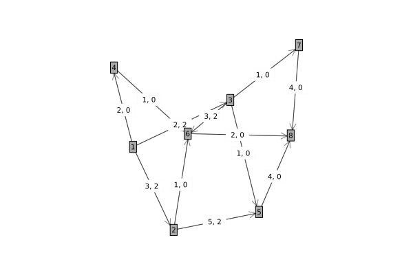Network Flow

The adjacency matrix can be formed from the non-zero entries in the matrix of maximum capacities between nodes, i.e.

\[G = \begin{bmatrix} 0 & 3 & 2 & 2 & 0 & 0 & 0 & 0 \\ 0 & 0 & 0 & 0 & 5 & 1 & 0 & 0 \\ 0 & 0 & 0 & 0 & 1 & 3 & 1 & 0 \\ 0 & 0 & 0 & 0 & 0 & 1 & 0 & 0 \\ 0 & 0 & 0 & 0 & 0 & 0 & 0 & 4 \\ 0 & 0 & 0 & 0 & 0 & 0 & 0 & 2 \\ 0 & 0 & 0 & 0 & 0 & 0 & 0 & 4 \\ 0 & 0 & 0 & 0 & 0 & 0 & 0 & 0 \end{bmatrix}\]

For example, the (1, 2) entry corresponds to a capacity of 3 and a minimum capacity of 2 from node 1 (row 1) to node 2 (column 2).

Similarly an adjacency matrix can be formed for the minimum capacities between nodes, i.e.

\[min_G = \begin{bmatrix} 0 & 2 & 2 & 2 & 0 & 0 & 0 & 0 \\ 0 & 0 & 0 & 0 & 2 & 0 & 0 & 0 \\ 0 & 0 & 0 & 0 & 0 & 2 & 0 & 0 \\ 0 & 0 & 0 & 0 & 0 & 0 & 0 & 0 \\ 0 & 0 & 0 & 0 & 0 & 0 & 0 & 0 \\ 0 & 0 & 2 & 0 & 0 & 0 & 0 & 0 \\ 0 & 0 & 0 & 0 & 0 & 0 & 0 & 0 \\ 0 & 0 & 0 & 0 & 0 & 0 & 0 & 0 \end{bmatrix}\]

We need to define the set of flow conservation constraints, i.e. the sum of the flows into a node must equal the sum of the flows out of a node except for the source node and destination node. The notation $I_{m->n}$ will determine the variables concerned. E.g. the conservation of flow for node 2 can be expressed as:

\[I_{1->2}*x_{1->2} = I_{2->5}*x_{2->5} + I_{2->6}*x_{2->6}\]

Data Acquisition

This is a simple toy problem setup. No data has been imported in this example.

Solve the problem

(i) We create a ConeQP object that represents the LP problem to solve cone_qp = get_qp(G, min_G).

(ii) We pass the ConeQP object to the solver solver = Solver(cone_qp).

(iii) Then when we're ready we call run_solver passing the solver object run_solver(solver)`.

(iv) We can access the solution by accessing the primal solution from the solver x = get_solution(solver).